Tingueu en compte que aquesta pàgina fa un tractament purament teòric sobre la capacitat de càrrega de les xarxes de ferrocarril. Els encreuaments i l'organització de la xarxa són molt més importants. Després d'aquest avís, anem a considerar els diversos factors que afecten la capacitat de càrrega de la seua xarxa

Distància entre senyals (DES)

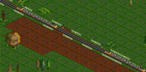
És un paràmetre obvi, relativament. Els senyals molts espaiats redueixen la capacitat de transport. Amb una distància entre senyals (DES) d'un senyal cada n caselles, l'espai disponible entre dos trens a màxima velocitat mai podrà ser inferior a n+1 caselles (figura 1); quan els trens estiguen tan pròxims entre ells que hajan assolit la densitat màxima teòrica possible. Tot allò en la pràctica és impossible.

Figura 1: L'espai mínim entre els dos trens és de 5 caselles, per a una distància entre senyals (DES) de 4 caselles.

Quina distància entre senyals (DES) he d'utilitzar?

Quina creu que és la distància òptima entre senyals? 1 senyal cada dues caselles? Un senyal per casella? O fins i tot menys? (En els trams diagonals cada casella compta com mitja).

Figura 2: Senyalització irregular. "Aquest buit pot causar problemes".

La llei de la major distància entre senyals

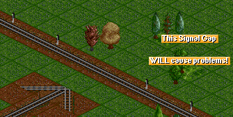
Per a qualsevol distància entre senyals que trie, ha de tenir en compte també la regularitat. La capacitat d'un tram de via es determina en primer lloc per la major distància que haja entre dos senyals d'entre tots els senyals que haja en aquest tram. Així, per exemple, en un tram amb un senyal cada dues caselles, si hi ha una anomalia de tres o quatre caselles sense senyals, es patirà una reducció de la seua capacitat i poden produir-se embussos en no cumplir la regla Núm. 1 (Figura 2). (Recorda que els senyals no poden col·locar-se als encreuaments, ponts i túnels. Per tant és inútil posar senyals cada dos caselles si després hi ha un pont de 12 caselles).

Figura 3: BAIX: Hem posat un senyal per casella. DALT: Hem posat un senyal cada mitja casella (en diagonal dues caselles compten com una).

Vies en diagonal

Com vostè ja haurà notat, les vies es construeixen en caselles de amb forma quadrada. Per defecte, el motor del joc considera que les vies en diagonal tenen una distància que equival a la diagonal d'una casella (√2=1,41). Per això els trens recorren menys caselles quan van per trams diagonals que quan van pels trams rectes (gràcies SmatZ!).

Figura 4: Teorema de Pitagores.

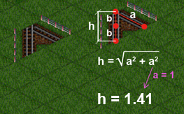
Com els trens es mouen més lentament (en considerar les caselles, no si parlem de distàncies) per les caselles diagonals, en aquests trams requeriran major nombre de senyals, (o reduir la distància entre senyals) per evitar embussos. La relació és d'1 a 1'41 (en aplicar Pitàgores). O siga que, 1 casella obliqua (h, a la figura 4) equival a 1'41 caselles rectes; i a l'inrevés: 1 casella recta (a, a la figura 4) equival a 0'7 obliqües.

Longitud dels trens (LT)

Es tracta d'una arma de doble tall. Un tren més llarg augmenta la probabilitat d'incórrer en una penalització de l'acceleració realista, necessitant així construccions més extenses i complexes. Però d'altra banda, un tren més llarg augmenta també la capacitat màxima de càrrega de la seua xarxa. Tinga en compte que si utilitza locomotores repartides entre el cap i la cua de tren, la mitja casella de pèrdua redueix encara més la baixa capacitat dels trens curts.

Els valors típics de LT són de tres a cinc caselles, quatre és especialment ideal per a xarxes d'alta velocitat (tenint en compte que normalment entren 2 unitats per casella, això significaria de sis a deu unitats, o 8 per a l'alta velocitat).

Pendent de traduir al català.

El text que segueix és l'original en anglès, pots col·laborar ajudant a traduir-lo al català.

Quantifying carrying capacity

Train Density (TD)

Your network will carry a certain number of trains, and assuming you have a standardised train length, we can define some metrics. The Train Density (TD) for a track is given in units of trains per thousand tiles, and can be calculated by counting the number of trains on that track and dividing by the length of the track.

Typical measured values for an unoptimized network of 4-tile trains are a TD of 25 (trains per 1000 tiles).

The maximum TD before traffic jams become self-propagating can be measured by permitting a queue of trains to accelerate from a halt and then measuring the train-train distance when all trains have reached full speed, and using the formula

1000 / (TL + train gap)

For example, a fully-laden 4-tile Chimaera (top-end MagLev (en)) was found to have a train-train distance of 12, giving critical density of 1000/16 or 62.5.

Because this critical density incorporates information about acceleration and time to reach top speed, it can also tell you about the practical capacity of your network. For example, using trains with a lower top speed actually makes it easier to have a dense network. The average train-train gap is much smaller for rail than for monorail or maglev. Repeating the previous example but using the electric rail T.I.M (en) gives a train-train distance of only 6, and a critical density of 100. Slow doesn't mean better, however, as the reduced line density will be more than compensated for by quick turnaround times.

It is possible to run a network at higher than the critical density, but it is ill-advised.

Theoretical Maximum Train Density

Simply put, this is the train density if your network is entirely filled with trains at the minimum distance between each other. You will never reach this.

This is given by 1000 / (TL + SD + 1)

For example, 4-tile trains and a signal distance of 2 will give a theoretical maximum train density of 140.

Carrying Capacity (CC)

Since TL alters the carrying capacity of a line, comparing TD across different TL is meaningless. In order to compare efficiency figures between different personal preferences, we need a new metric. This new metric will simply be a measure of how many units of cargo your network is transporting per year, per track. It will be directly proportional to the average quantity of cargo per track tile, and also to how fast this cargo is moving.

Work on this unit is pending.

Making your network more efficient

Ok, so now that we've defined the parameters that we had already intuitively understood, how can we use them to improve our networks? The golden rule of network optimisation is that trains on the network never slow down. There are two possible parts of a network where this could happen, splits and merges.

Splits

For a track split, one must ensure that there is not a longer-than-normal signalling gap at the split point. This can be taken care of by careful or over-abundant signalling.

Merges

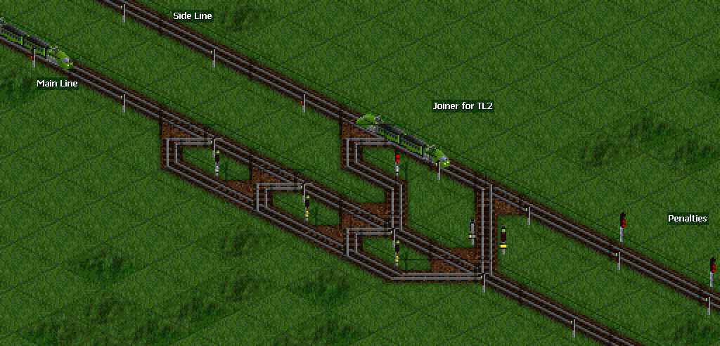
Merges present us with a unique problem. For a trivial merge, trains on the mainline could potentially be stopped by a sideline train. There is already a body of work on Priorities by our colleagues in the cooperative circuit. A perusal of this link should familiarise you with the principles of priority merges.

Consider a typical non-junction merge, at the exit of a pickup station. A tightly-packed optimised stream of trains enters the station, but because of differences in loading times, this order is disrupted on the station exit, and you end up with two tracks of loosely-packed trains. One of these lines, designated the main line, will have, on average, train-train gaps large enough to fit a third train into. Simply connecting the two lines together will not work, and a priority merge is required.

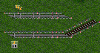
Note that, because trains that drop off cargo always spend the same length of time at a platform, it is possible to dematerialise and reassemble a tightly packed stream of trains, even one above the critical density! (Figure 3)

🔍

Figure 3: Dropoff with stream reassembly

A first-pass merge using a priority block will reduce the traffic ratio from 1:1 to about 3:1 in favour of the main track (Figure 4). Adding a second priority merge straight after the first one would be a futile gesture, since trains on both lines would continue at the same speed and the mainline train would simply claim priority again. Introducing a delay by a loop of track, followed by a second priority merge, will reduce the sideline to a mere trickle of trains and will have filled in most of the available slots on the mainline. Existing solutions would involve a pre-acceleration track, however a cyclotron eliminates the need to lose momentum.

Figure 4: Priority merge

Cyclotrons

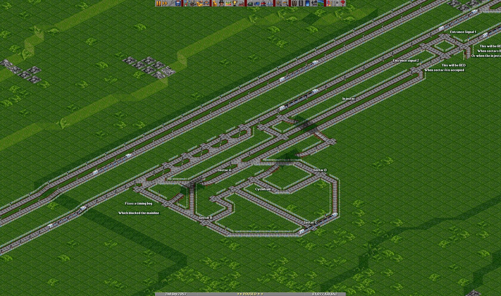
Consider a sideline that loops back on itself after a failed priority merge. A train in this loop would continue to re-test the mainline for entry conditions, once every 8 * 'TL tiles until it found a space large enough to merge with the main line. After the cyclotron was empty, the next waiting train could pre-accelerate and be injected into the cyclotron, ready to continue the cycle. This system has some flaws, however, as it has a capacity of one train and there will be many missed opportunities due to the train being in the wrong position in the accelerator. [Broken link to Simple Cyclotron removed.] Junctions are a large and well-trodden area of openttd; I have restricted myself to unbranched feeder structures. You will find that a highly-optimised stream of trains does NOT weather a junction well.

Refinements to the cyclotron are possible. There is enough space on the track loop to contain two trains, and a system of priority signals will enable a second train to optionally enter the cyclotron. With two trains in the cyclotron, there will be a doubled chance of entering a slot on the mainline. In order to prevent a traffic jam inside the cyclotron (which would be disasterous), some delay tweaking is necessary, but the end result is exceedingly useful.

The injection delay assumes that the second injected train is accelerating from standstill, and there is a small chance that second train has in fact chanced upon the cyclotron entrance at full speed. In this case, the timing will be wrong and the second train will almost certainly cause a jam within the cyclotron (and consequently on the main line). This can be compensated for by some additional signalling to filter out full-speed trains. The filtered out full-speed trains can either be diverted onto a second loop, or simply drained of momentum by a signal.

A cyclotron incorporating all the optimisations discussed, and some additional fixes, is shown in Figure 5.

🔍

Figure 5: full-featured cyclotron

[Broken link to a savegame removed.]

Editor's note: Whilst I would like to defend my cyclotron refinements, experimentation has proven that pre-acceleration is a more robust system. The two have been combined in the savegame linked previously.

Feature availability

<1.0
☑

1.0-1.2
☑

1.3
☑

1.4
☑

1.5-12.0
☑

Nightly
☑

Parallel cyclotrons

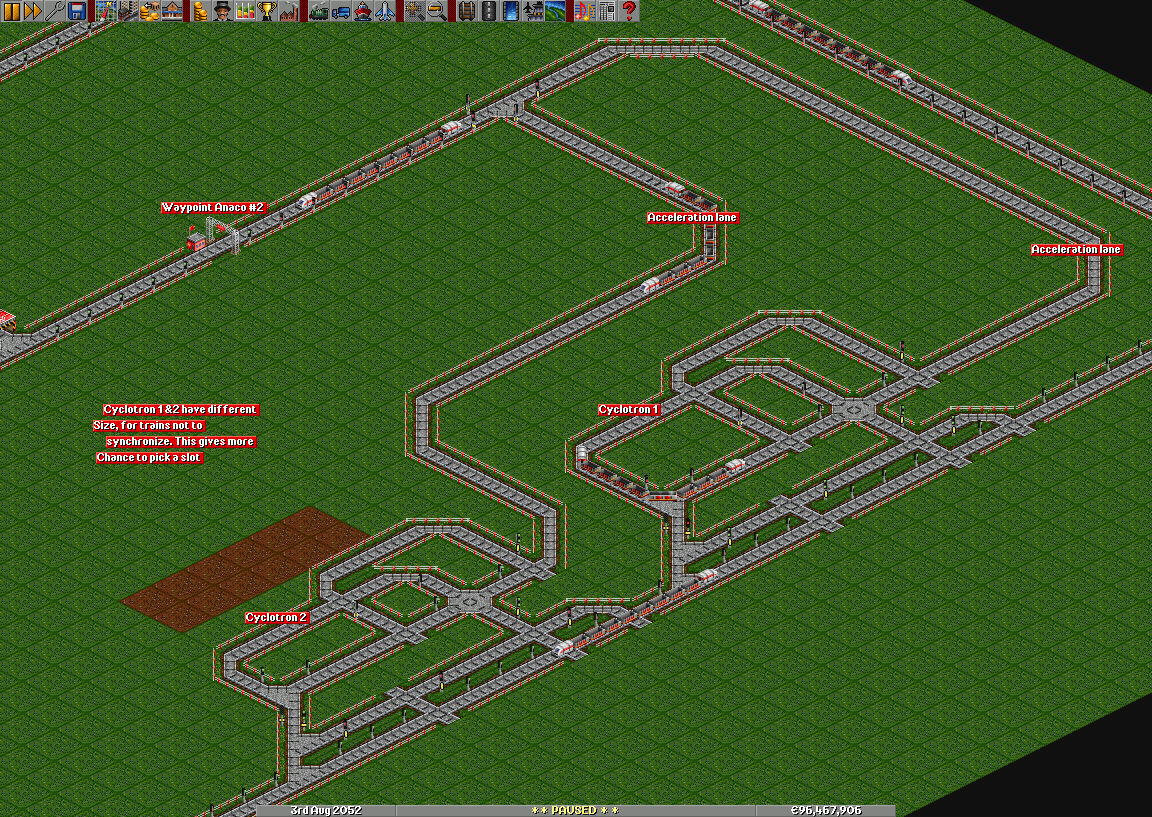
An attempt to minimize the drawbacks of the full featured cyclotron leads to parallel, small, 1-train cyclotrons. In this design, an array of cyclotrons, each handling one train, may be fed simultaneously. They may have different loop size in order to prevent synchronization between the cycling trains, giving more chance to find a slot in the flow of the main line. Each loop still needs it own acceleration lane so the trains enter the loop at full speed. If a train happened to enter the loop at low speed, it would get a chance to join the main line at non-max speed and cause a possibly large traffic jam.

Figure 6 shows a parallel cyclotron with two loops.

🔍

Figure 6: Parallel cyclotron

A savegame with the example given in Figure 6 is available Here (version 0.7 or higher required to open).

Advantages over the full featured cyclotron:

Can handle more than two trains
Faster fail-and-retry pace
No need to synchronize the looping trains
Easier to build and remember

Drawbacks:

Bigger when using more than one loop

Categories:

Folder: Community

Contents

Capacitat de càrrega de la seua xarxa